How to Continue a Rule Google Sheets on Mobile

Google Sheets offers a lot of advanced capabilities that help extract meaning from a pile of data. One of them, simple and at the same time powerful, is conditional formatting. It helps turn bland rows and columns of black text on white backgrounds into a colored and visually appealing dataset. This saves time and also makes the data more readable and meaningful.

What is Google Sheets сonditional formatting?

Google Sheets conditional formatting is a feature to automatically change the font properties of a specific cell, row, column, and even the background color of the cell, based on rules you set. In other words, this tool uses the power of visualization to make your data stand out. By coloring cells, you highlight specific values, making them easier to view, and easier to understand complex tables. With conditional formatting, data becomes more visually appealing and therefore, human-readable.

When you can apply conditional formatting in Google Sheets

Conditional formatting can be used in practically any workflow to visualize information: patterns of data, trouble spots, good news, or even faulty or flawed data. It is possible that no other Google Sheets tool can be used in so many applications.

• Sales managers need to gain quick insights from a huge amount of sales data => they use conditional formatting.
• Accountants want to highlight all negative values in red in their profit/loss calculations => no problem, they apply conditional formatting.
• Project managers try to understand their resource utilization=> again conditional formatting can come to the rescue.

It also serves as a great way to track goals, giving visual indications of the progress against specific metrics. And that's not to mention daily and weekly reports, which are in abundance in large organizations. They can become a real pain if you are busy and they are not conditionally formatted, hence, not meaningful at first glance.

So, conditional formatting can come in handy whenever you would like to liven things up in your Google Sheets tables.

How to use conditional formatting in Google Sheets

Before getting into detail, it is important to understand that any work with conditional formatting follows the same pattern, which has three key elements:

• Range. This is a cell or cells to which the rule should be applied.
• Trigger. It defines the condition for the rule to be used. For example, the trigger can be Less than.
• Style. When the rule is applied, it changes the cell to a style of your choosing.

The steps to follow are:

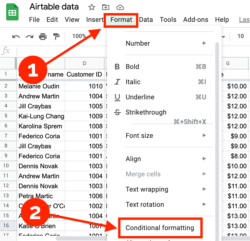
1. Click Format > Conditional Formatting.
2. Select a range.
3. Set conditional formatting rules
   • Select your style under Formatting style.
   • Select your trigger from the Format cells if… dropdown list.

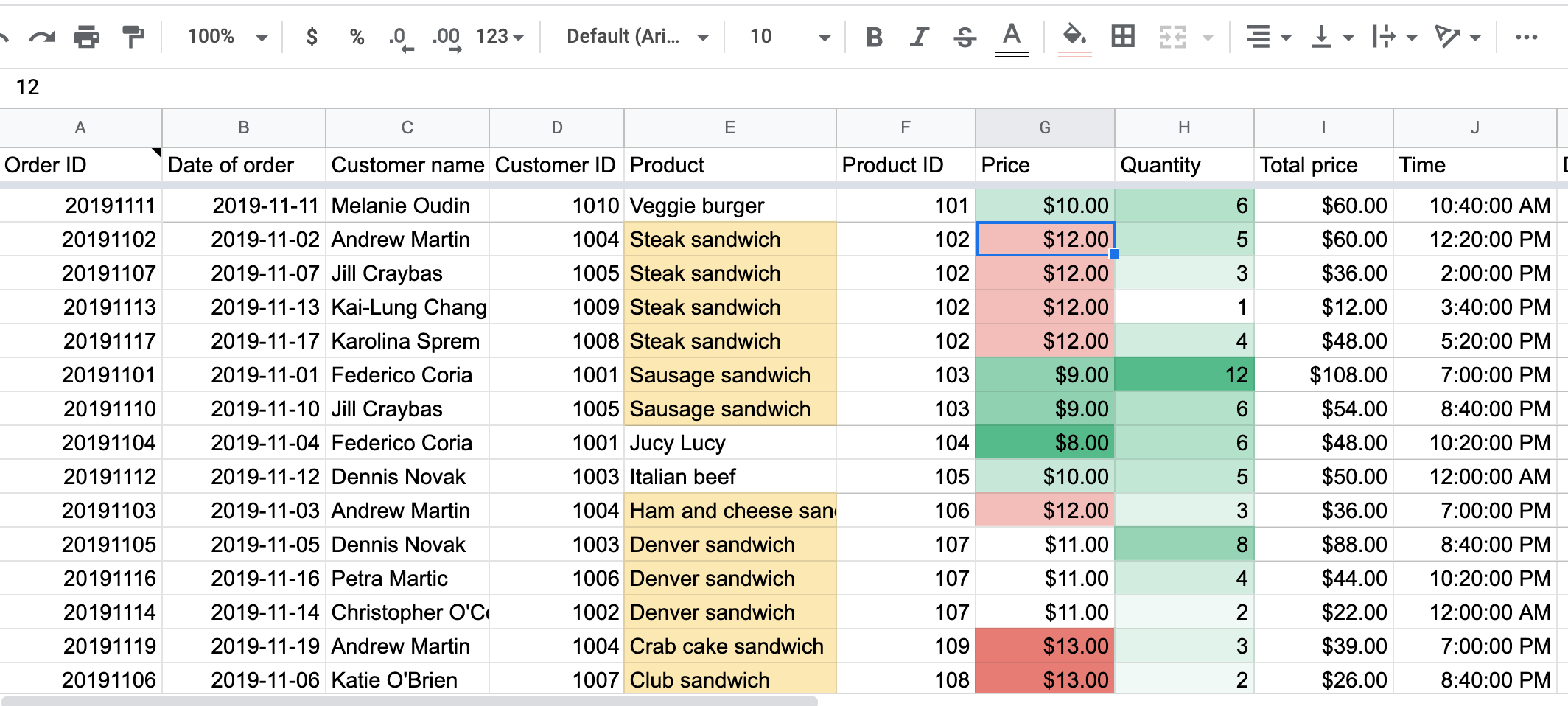
Let's consider each step in more detail. For that, we'll use a dataset that was imported from Airtable to Google Sheets with the help of Coupler.io.

Coupler.io is a data integration solution to automate data exports from different apps such as Pipedrive, Jira, HubSpot, and many others to Google Sheets. In addition, you can use the Google Sheets integration by Coupler.io to combine data from multiple sheets into one without any formulas.

Check out the list of Google Sheets integrations available.

Step 1. Click Format > Conditional Formatting

The first step is pretty straightforward and logical.

Step 2. Select a range

As for the second step, you have two options here:

Option 1: Select a range (cells, columns, or rows) and then click Format > Conditional formatting. This will pop up a conditional formatting toolbar on the right side of your screen. If your data range is small, this is the way to go.

Option 2: Click Format > Conditional Formatting and then enter your range under the Apply to range tab. This is especially comfortable when you work with large amounts of data, and there is a risk that you may make errors when selecting a range.

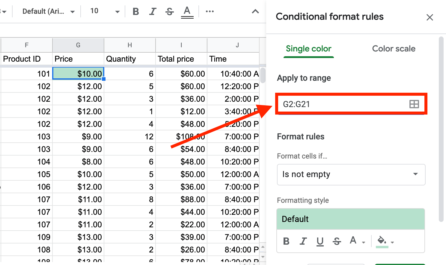
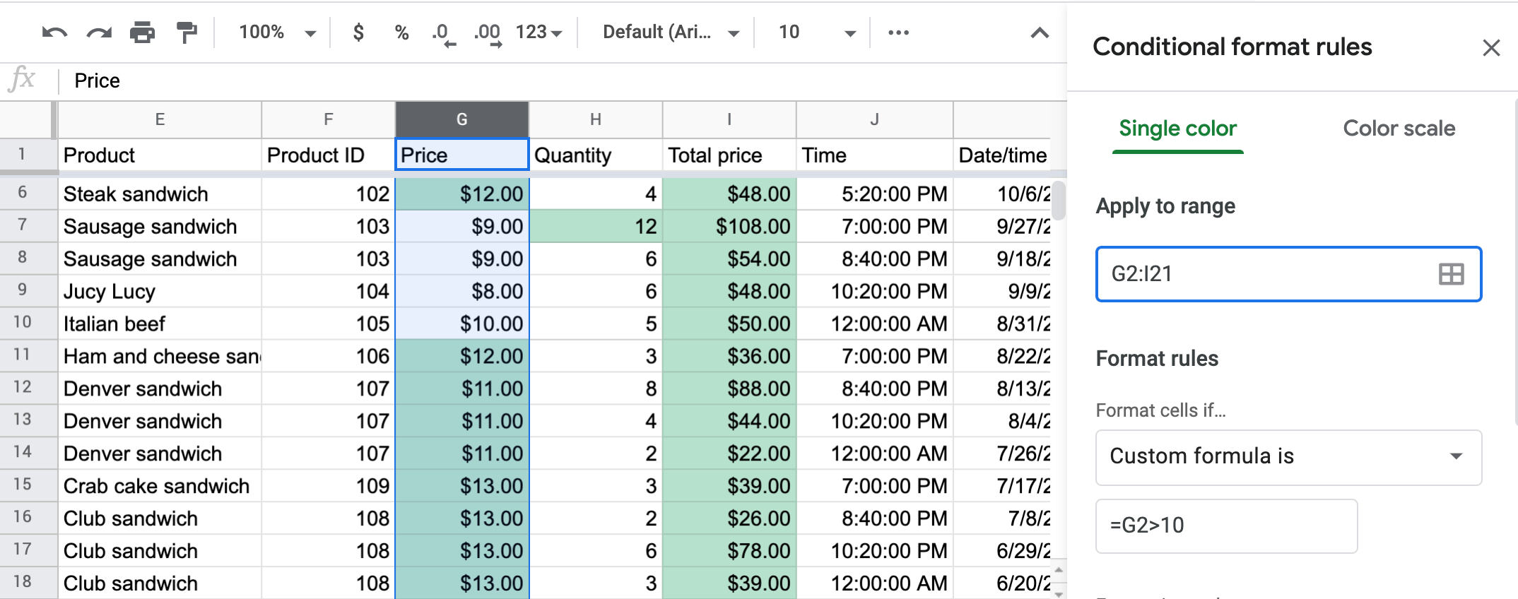
If you target a range of cells, you should enter the first and last cell in the range and separate them by a colon, as G2:G21 in the example above. If you need to highlight a single cell, enter the cell tag instead of the range (e.g., G2).

You may also need to work with multiple ranges. The easiest way to do this is to click the icon to the right of the range field and select Add another range.

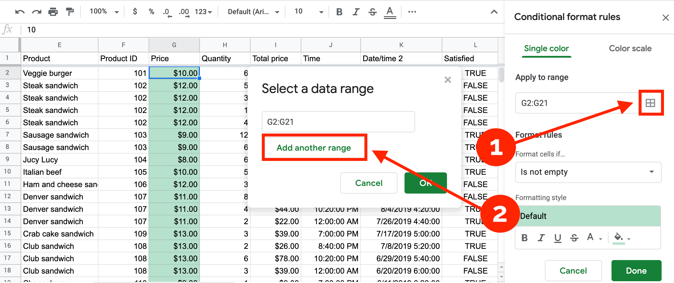
For example, I chose the H2:H21 range to be colored.

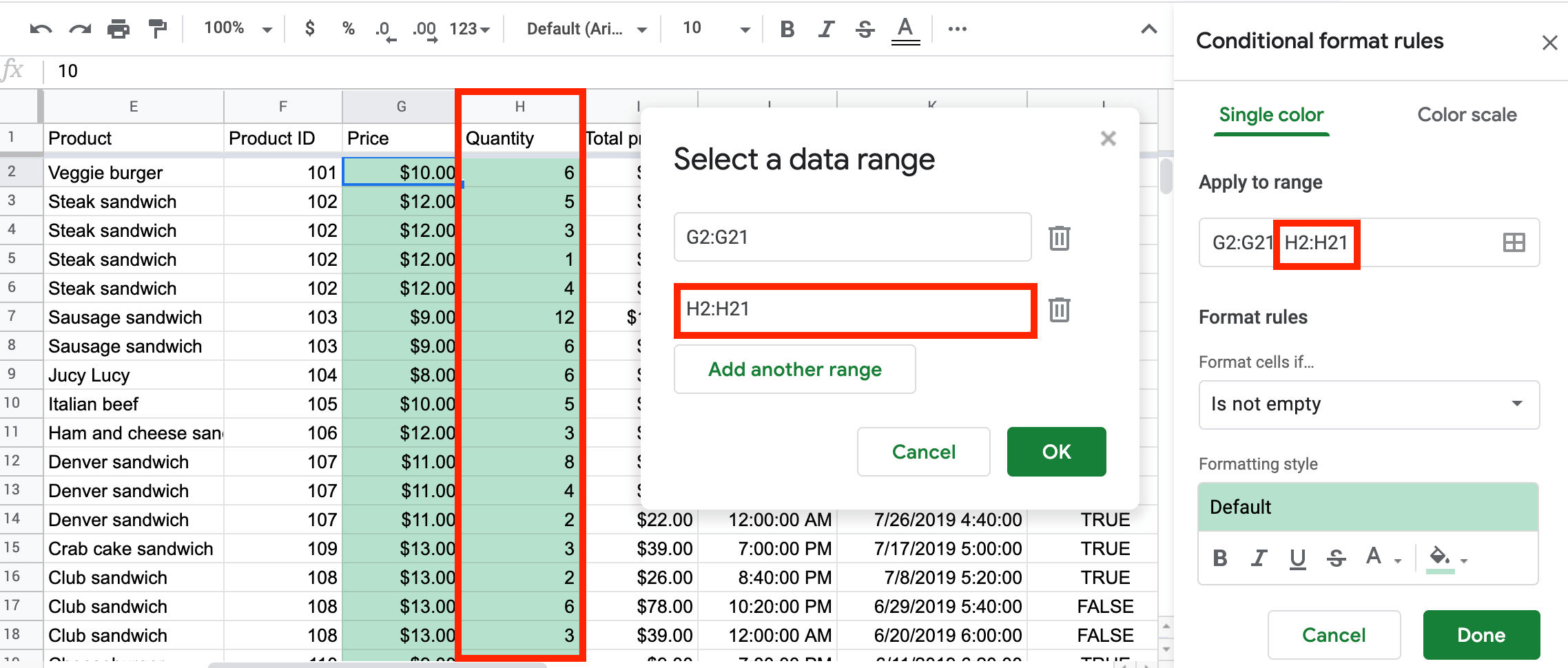
In this way, you can highlight as many ranges as you like.

Step 3. Set conditional format rules Google Sheets

Formatting style

The next thing to do is to select the style. It might seem counterintuitive to skip Format cells if… and start with the style first, but the moment you set the condition, your cells will change the style. That's why it seems more convenient to reverse the order, although the end result is the same.

To select a style, click Default under Formatting style,

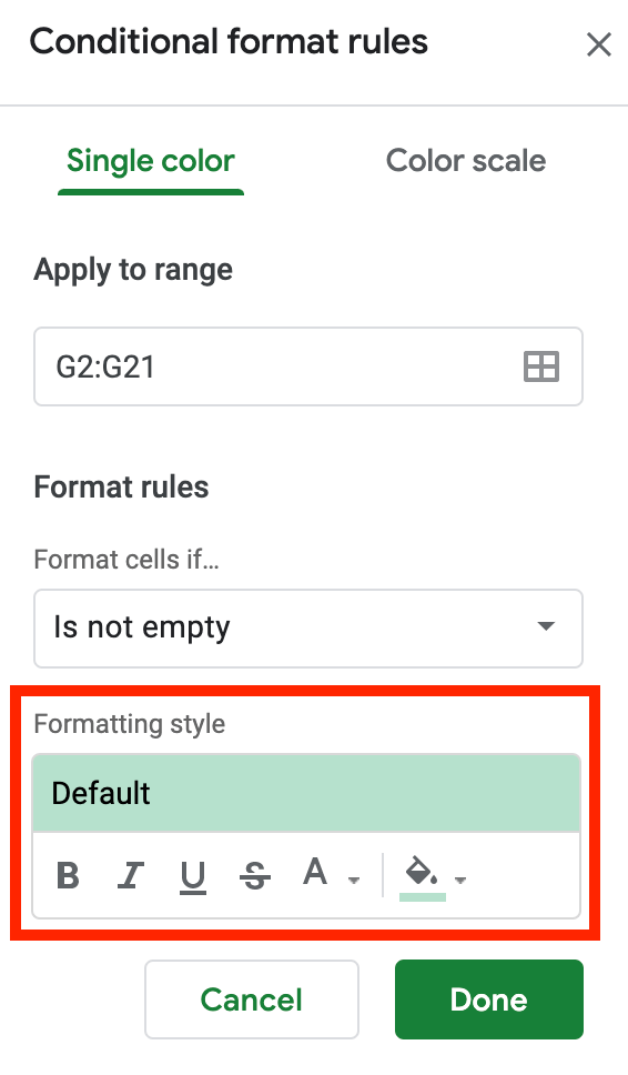
and you'll see the default style options.

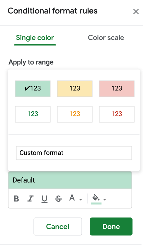
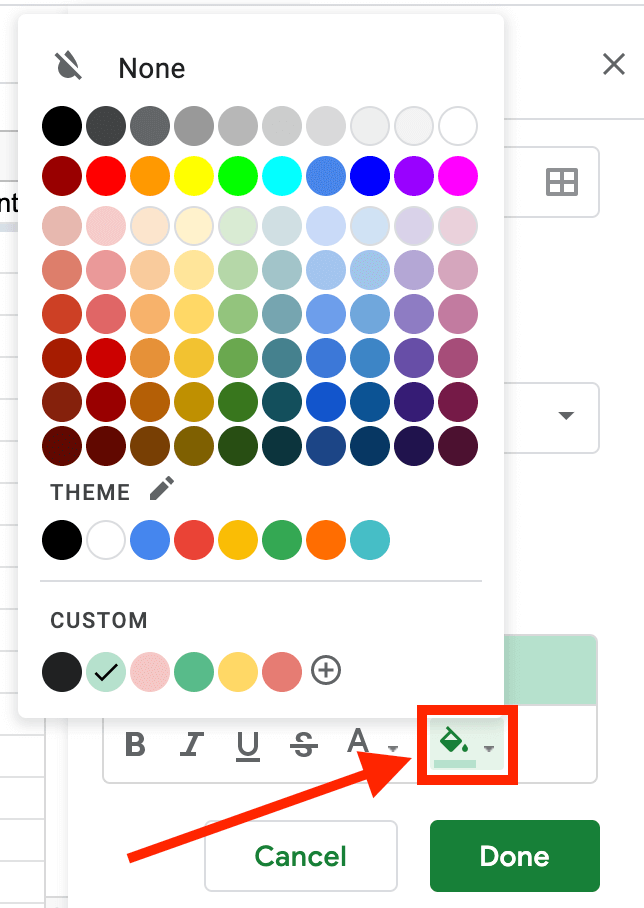
If none of these options looks attractive to you, create a custom style. You can choose the text style to be bold, italics, underline, or strikethrough, and you can select your font color and cell background color by clicking the color selection button.

Format cells if… – select your trigger from the drop-down list

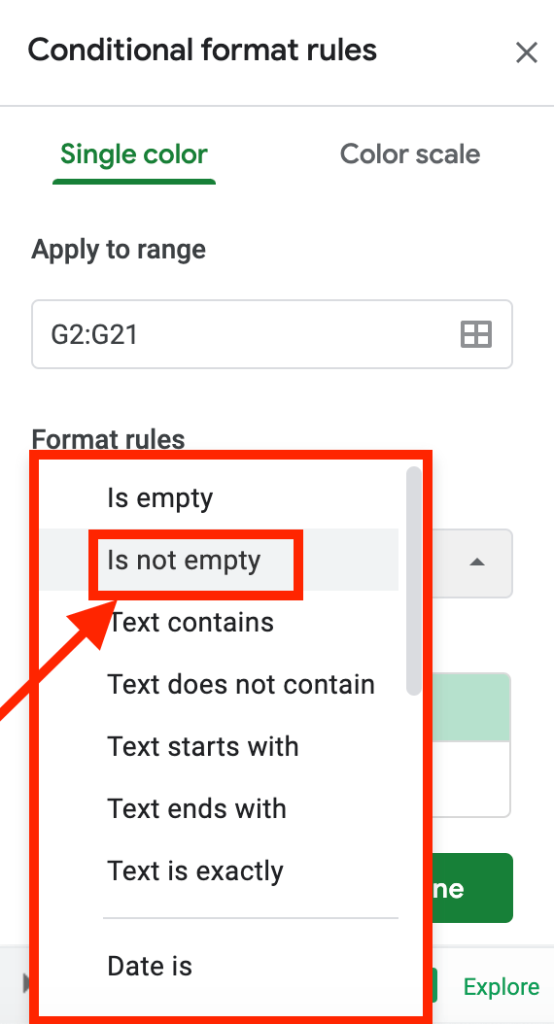
Let's have a look at how the conditional part of the formatting works on a case-by-case basis. The trigger (Format cells if…) defaults to Is not empty, but clicking it will drop-down a list of many rules that you can apply to conditional formatting in Google Sheets.

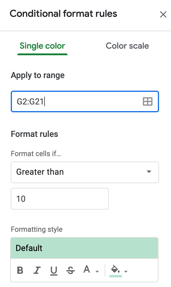
For our first example, let's pick Greater than from the dropdown options, and apply the rule Greater than $10 to the range G2:G21, the product price column.

Let's also use colors to make the numbers even more explicit and meaningful. For that, we'll apply two separate rules:

1. Mark green all values that are greater than 10
2. Mark red all values that are less or equal than 10.

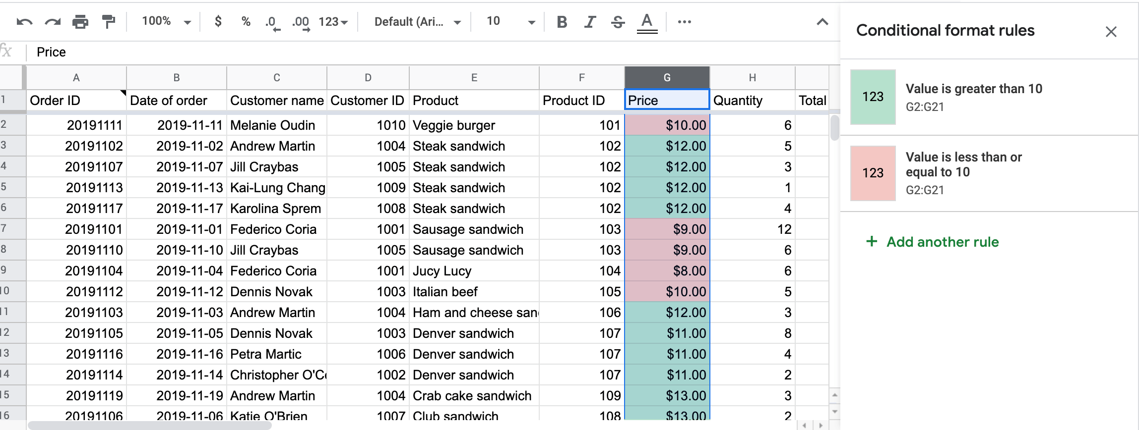
And yes, remember to click Done every time you want your rules to be applied:).

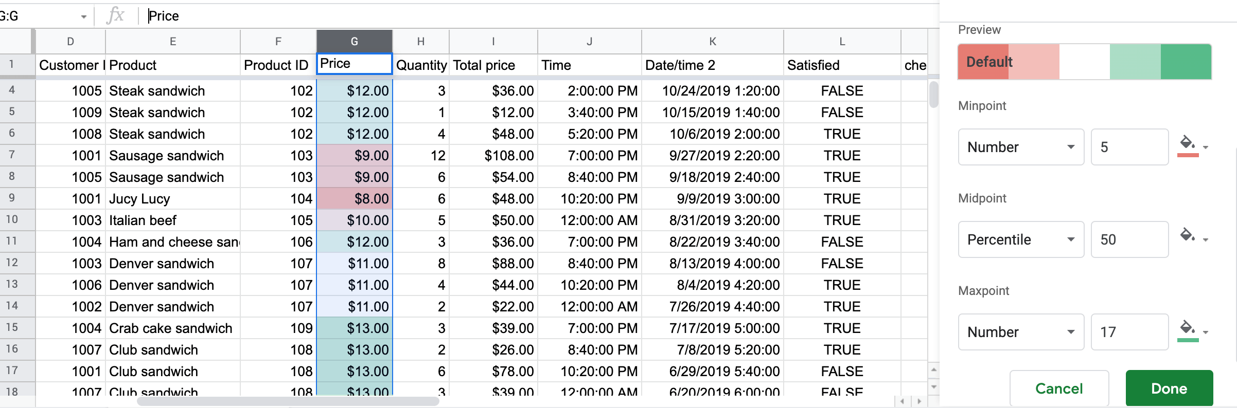
Google Sheets conditional formatting color scale

Another great thing about coloring your cells is that you can use a color scale to make your data look even more meaningful and visually appealing.

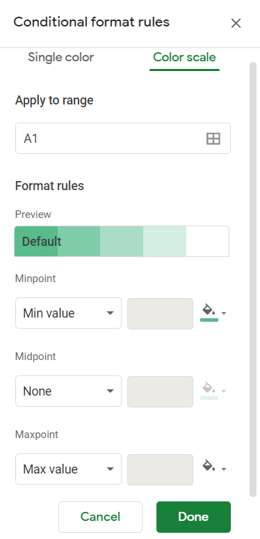
By default, Google Sheets will use the color scale between the minimum and maximum values, but you can change the way your scale looks by setting custom maximum and minimum numbers.  For example, you may want to have something like this:

Custom conditional formatting in Google Sheets using Custom formula is

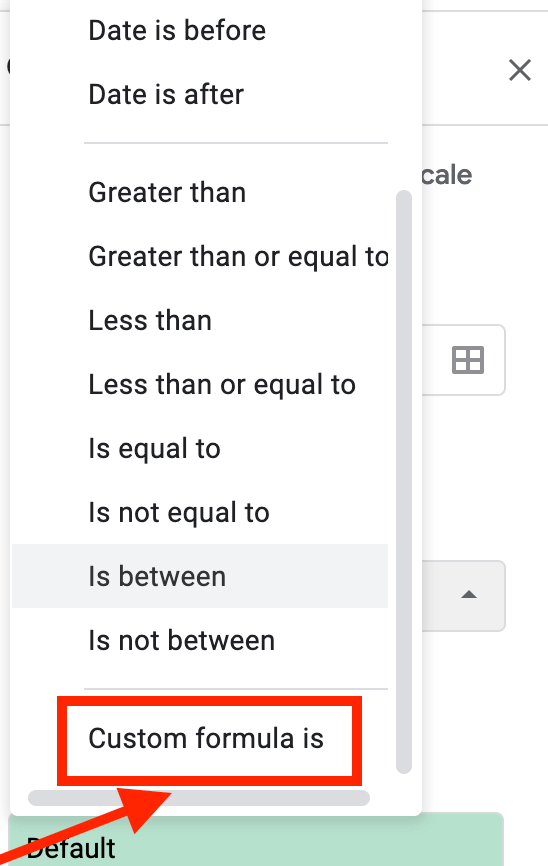
There are many options offered by the Format cells if… option, but probably one of the most useful is the custom formula option. The possibility of entering a custom formula allows you to be more flexible with your data and broaden the scope of available manipulations.

To access it, you need to select the dropdown under the Format rules, then scroll to the bottom and choose "Custom formula is…"

Keep in mind that all custom formulas start with an equal sign (=). Also, if you are used to using AND and OR functions in your regular Google Sheets formulas, the good news is that they work in conditional formatting as well.

Conditional formatting in Google Sheets – other format rules examples

Let's take a step further and consider some other, more complicated cases which are more frequently used in real-life.

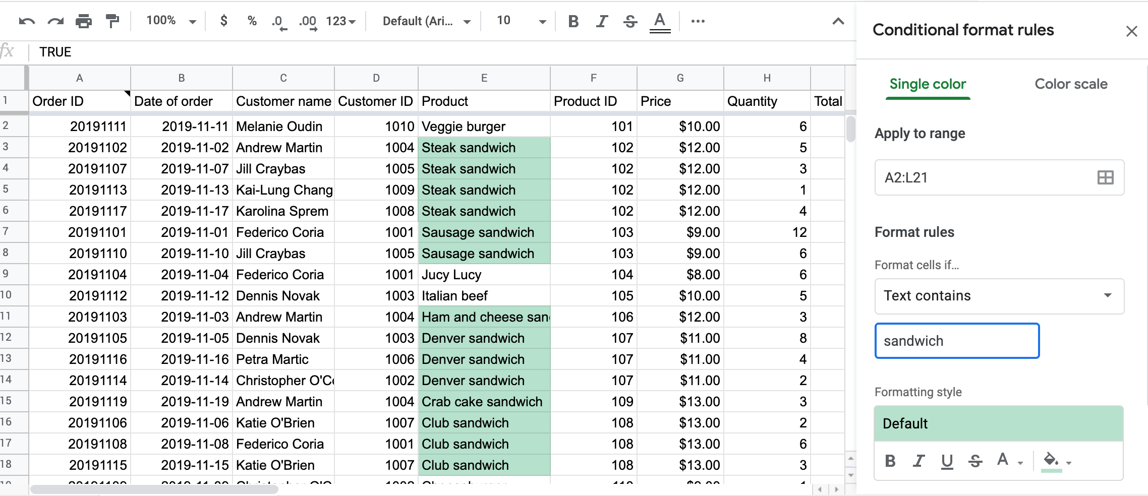
Google Sheets conditional formatting rule – text contains

Often, you may want to find or highlight a word or words in your data sets. It is easy to do with a text-based rule – a cell will change based on the text you type into it. The options for a text-based rule are:

• Text contains
• Text does not contain
• Text starts with
• Text ends with
• Text is exactly

For example, let's say you want to see what kind of sandwiches there are on the menu. In this case, you may either select the whole table (as in my case) of your product column and choose Text contains and type "sandwich". All kinds of sandwiches will be highlighted.

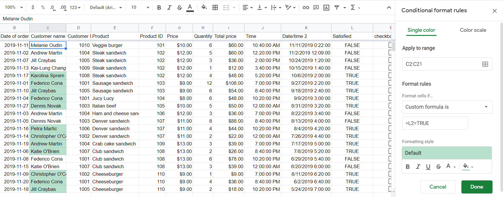
Google Sheets conditional formatting based on another cell value

Sometimes you may also want to apply conditional formatting based on another cell. Let's say you want to find out which of your customers were satisfied with the products. That's where the custom formula option comes in. The formula to apply is

=L2=TRUE

So, whenever conditional formatting checks a cell in the range C2:C21, it checks the condition =L2=TRUE, where L is the column with values that show customer satisfaction.

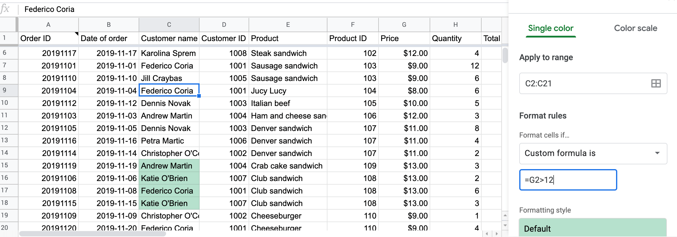
The same logic can be used if you need to find out who buys the most expensive products, in our case $13. The formula for this is

=G2>12

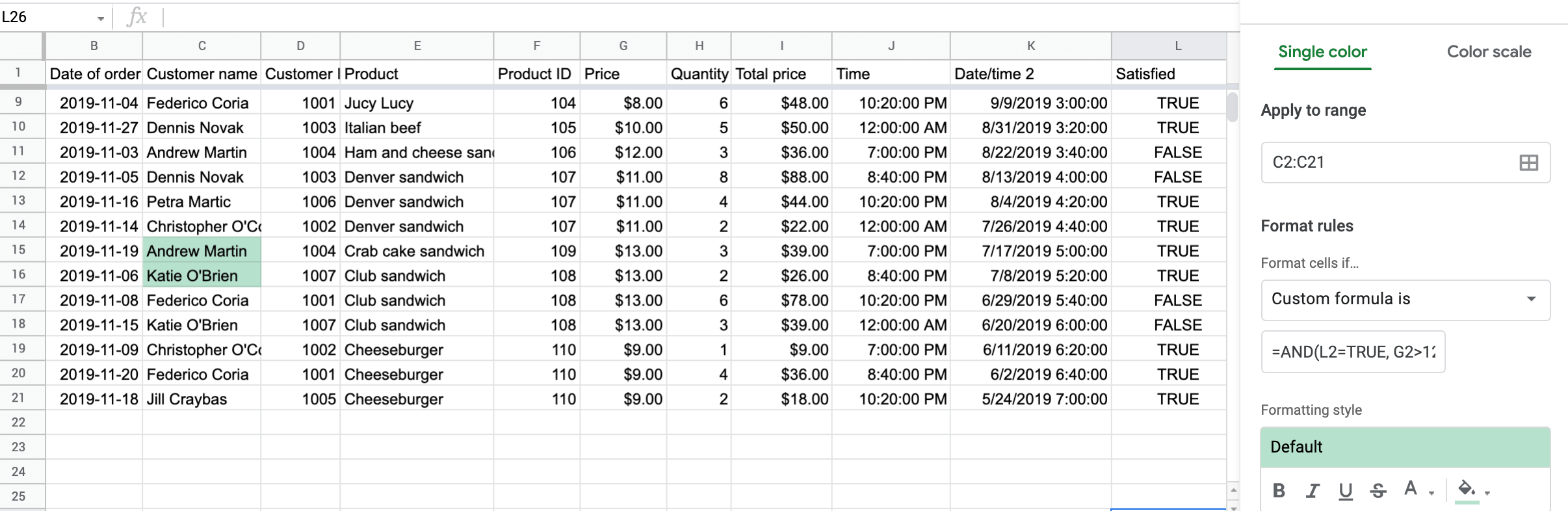
If you need to make your selection even more targeted, then try using AND or OR functions. For example, the following formula will highlight customers who buy the most expensive products and are completely satisfied.

=AND(L2=TRUE, G2>12)

How to conditional format an entire row in Google Sheets

But what if you want to highlight the whole row, based on a cell value? Let's say you want to check what your most picky customer Federico Coria buys. Again, choose Custom formula is… from the drop-down and type:

=$С2="Federico Coria".

Any row that has Federico Coria in the column will be highlighted.

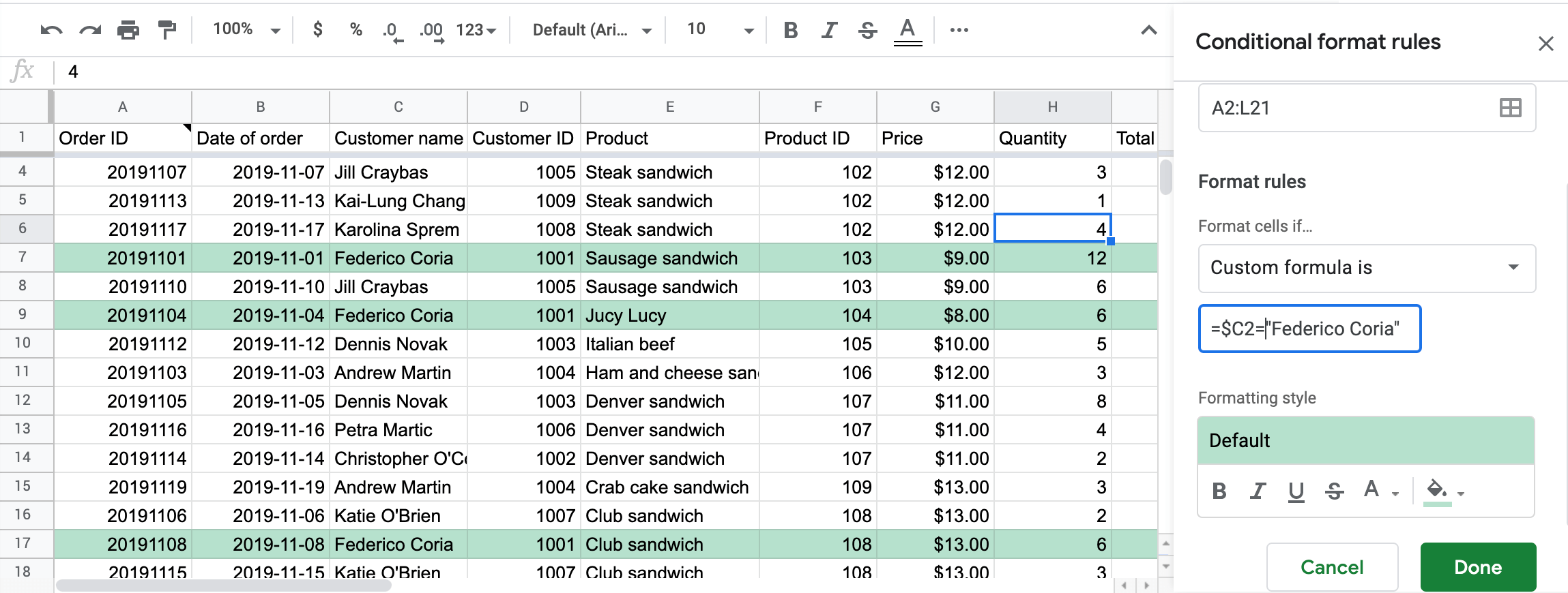
Just keep in mind to select your entire data set, in our case, A2:L21.

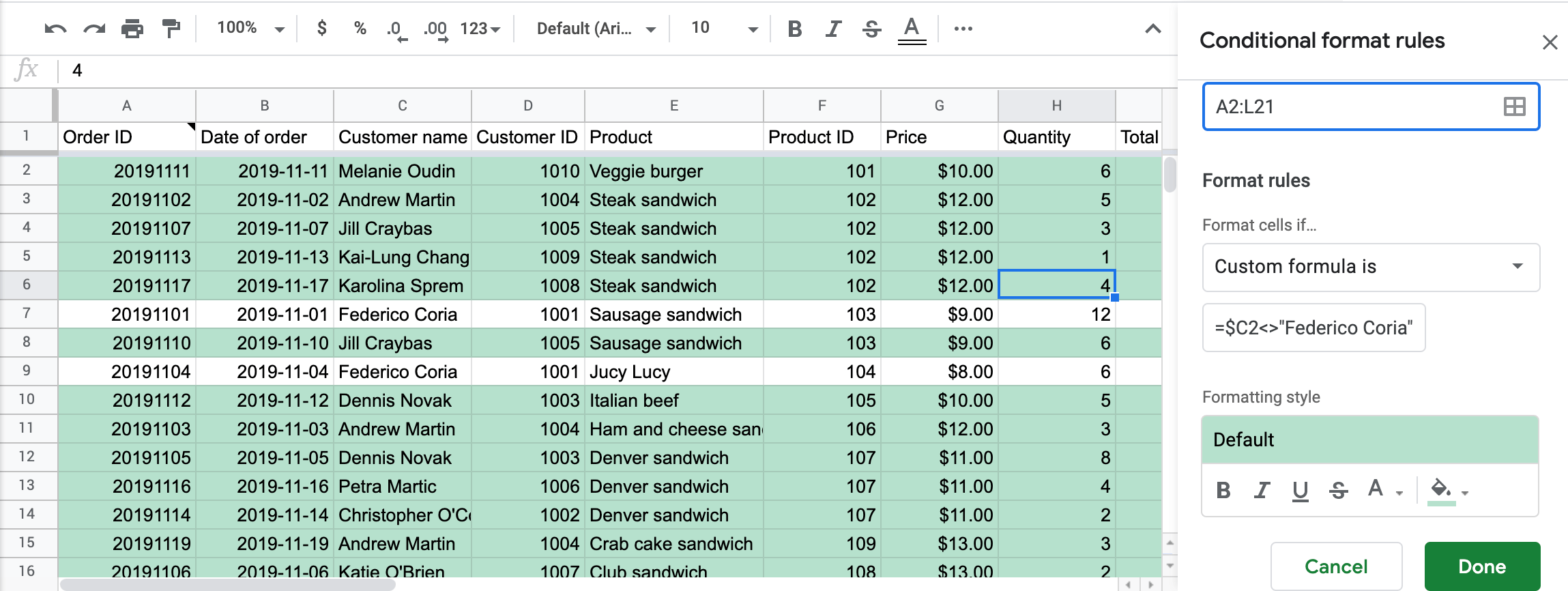
Almost the same should be done if you want to highlight any rows that don't include a given value. Replace = with <>. In our case, the new formula will look like this:

=$С2<>"Federico Coria"

Highlight alternate rows with the help of conditional formatting in Google Sheets

Zebra lines are often used when the reports are to be printed out. It helps increase its readability and gives it a more professional look.

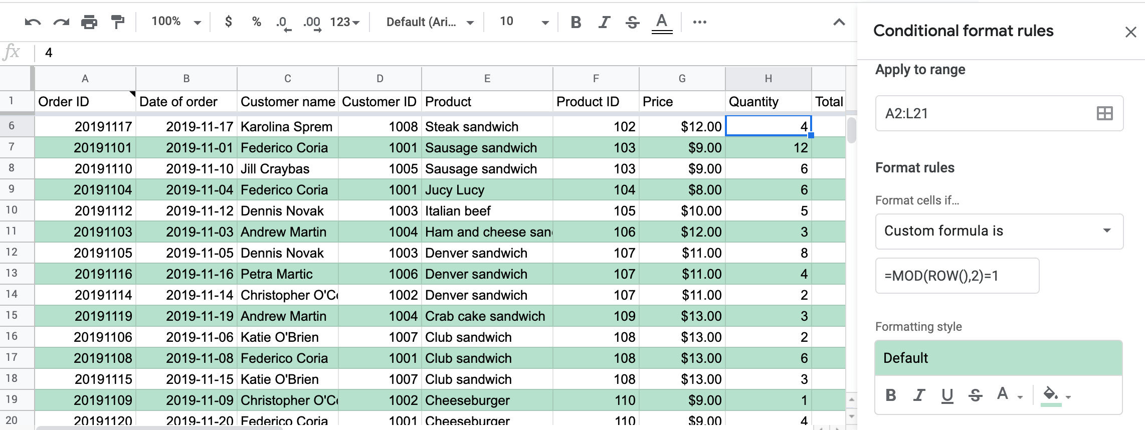
To highlight alternate cells, follow the already familiar algorithm. Keep in mind to select the whole dataset and, in the Format cells if… drop-down, select the Custom formula is option. The formula to enter is

=MOD(ROW(),2)=1

This will highlight alternate rows in the selected range.

How it works: The ROW() function returns the row number of a given cell. The MOD() function then divides it by 2 and returns the remainder. When the remainder is 1 (if there is an odd number of rows), the condition is TRUE, and the conditional format is applied.

If you want to highlight an even number rows, use:

=MOD(ROW(),2)=0

Сonditional formatting for duplicates in Google Sheets

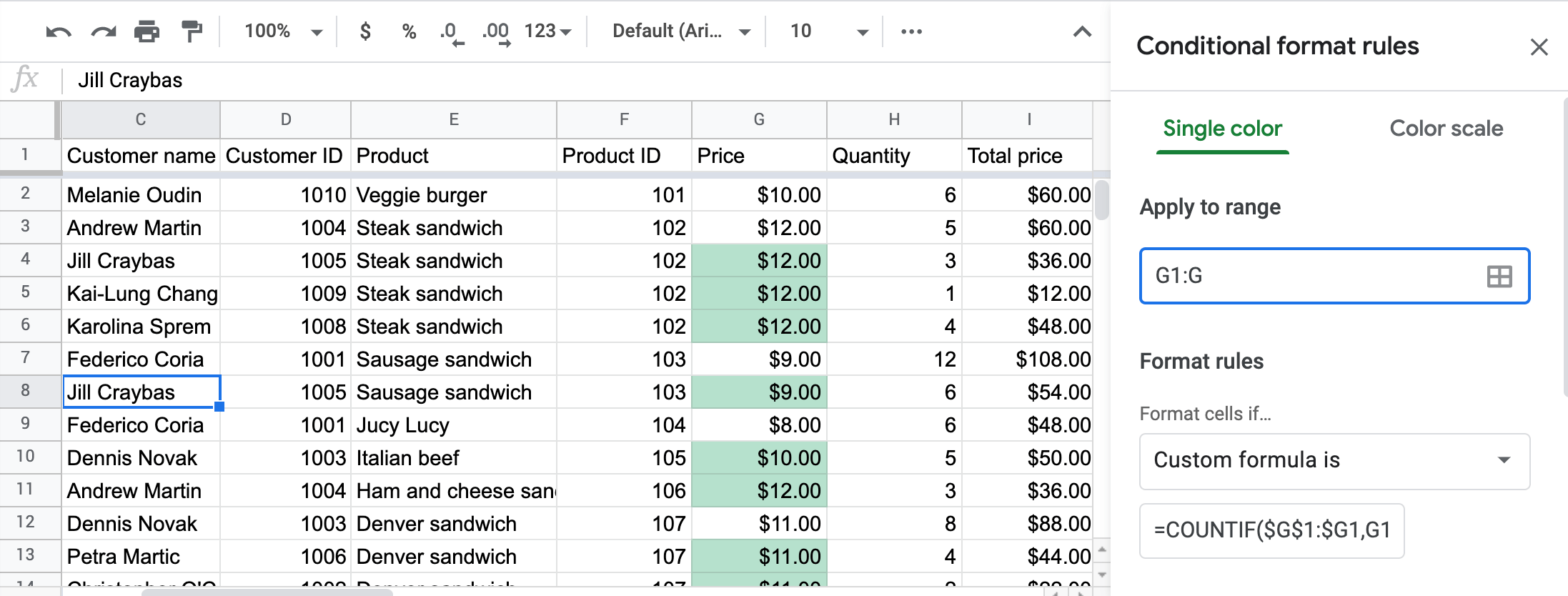
Sometimes you may need to see duplicates in your Google sheet – for example, to be able to delete them. With conditional formatting functionality, you can't actually remove duplicates, but you can identify and highlight them. For this, you need to use Custom formula is as a formatting rule and apply a COUNTIF formula for a selected data range. For example, to identify duplicates in the column G1:G, the following formula will do the job:

=COUNTIF($G$1:$G1,G1)>1

Read our blog post to learn more about how you can highlight duplicates in Google Sheets.

Conditional formatting for dates

Here is an example of date-based conditional formatting:

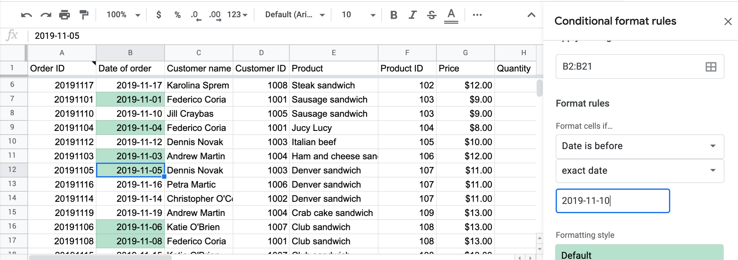
We highlighted the cells that contain values before the specified exact date value. You can also use conditional formatting based on relative dates (today, tomorrow, yesterday, in the past week/month/year). Read our blog post Google Sheets Date Format to learn more cases for highlighting dates.

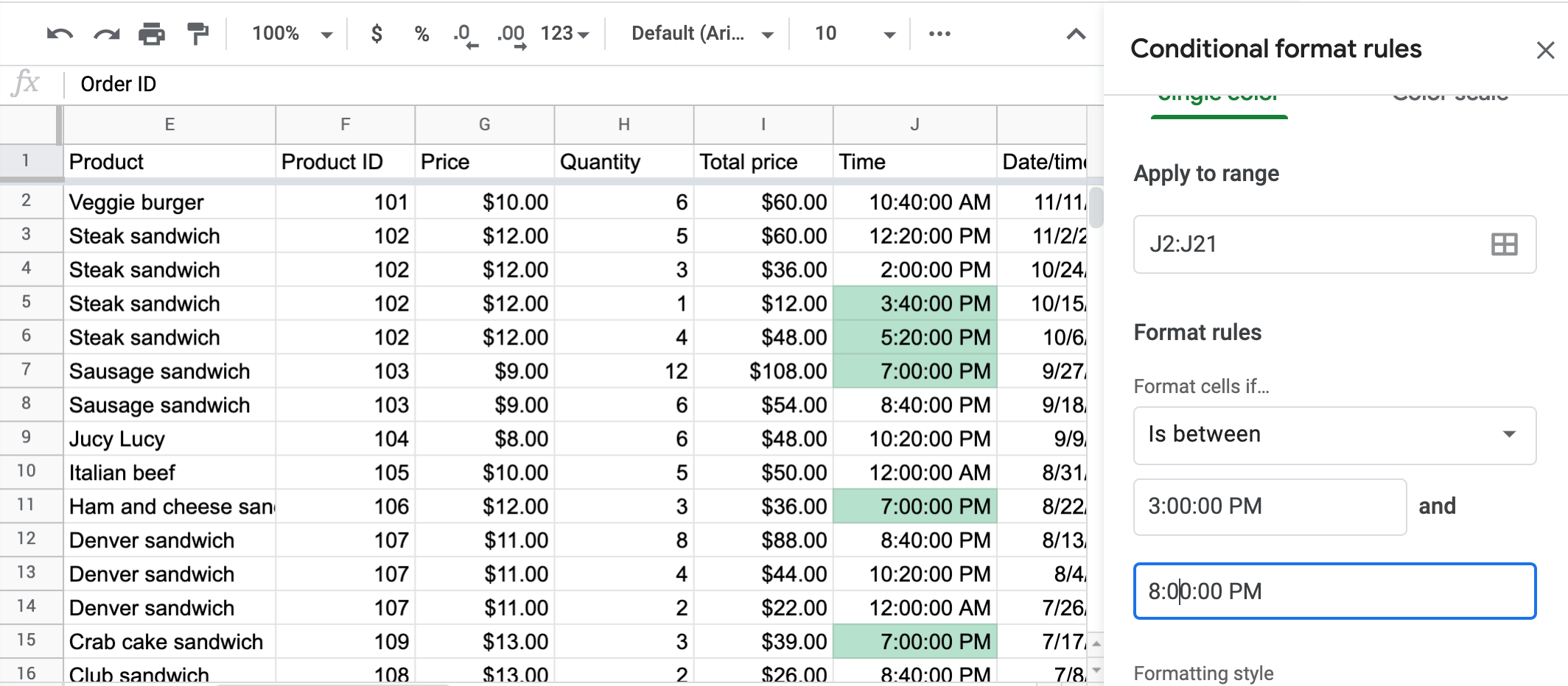
Google Sheets conditional formatting based on time

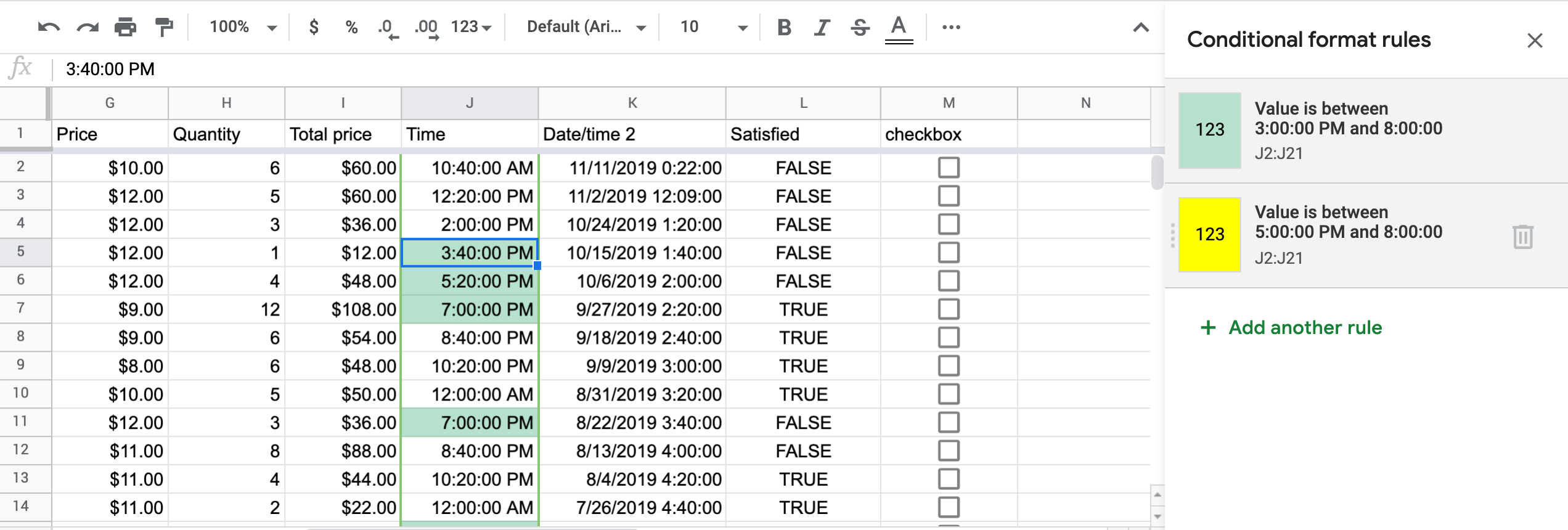
You may also want to conditionally format your sheet based on time. It is easy to do if you have time as a separate column, as J column in the demo sheet. Then, you may choose any condition that applies to numbers. For example, if you want to highlight cells that are between 3:00:00 PM and 8:00:00 PM, you need to choose Is between from the drop-down and enter your values.

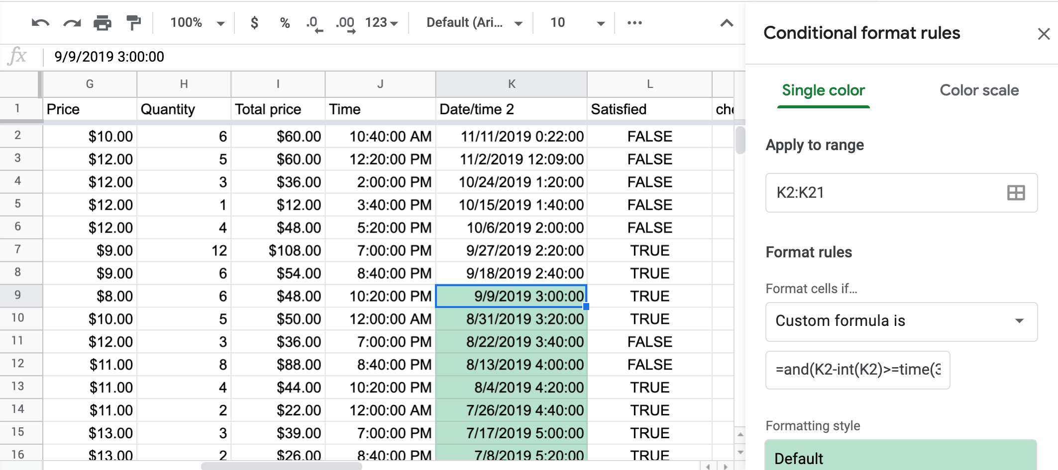
If your time is not in a separate column, but, let's say, combined with date, things won't get any easier. In that case, you need to choose Custom formula is and enter the following formula:

=and(K2-int(K2)>=time(3,0,0),K2-int(K2)<=time(8,0,0))

Google Sheets conditional formatting with multiple rules

As we've already mentioned, it is possible to set up multiple conditional formatting rules in Google Sheets. A reminder that you have to use the Add another rule button below your conditional formatting rule. Below you can see how it looks in practice.

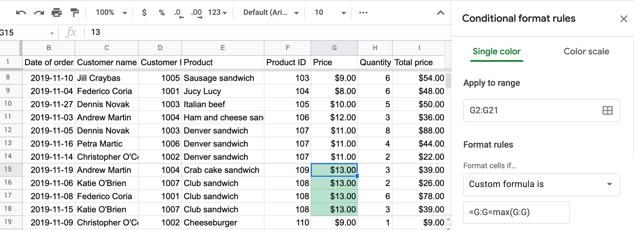
How to highlight the lowest or highest value using conditional formatting

It may also be useful to know how to highlight specific values in a spreadsheet. Let's take a look at how you can identify the lowest and highest values. You have to follow the same, hopefully already familiar algorithm, and in the Format cells if drop-down list, select the Custom formula is option. The formula to use for the highest value is

=G:G=max(G:G)

• G stands for the column where you want to search for the highest value.

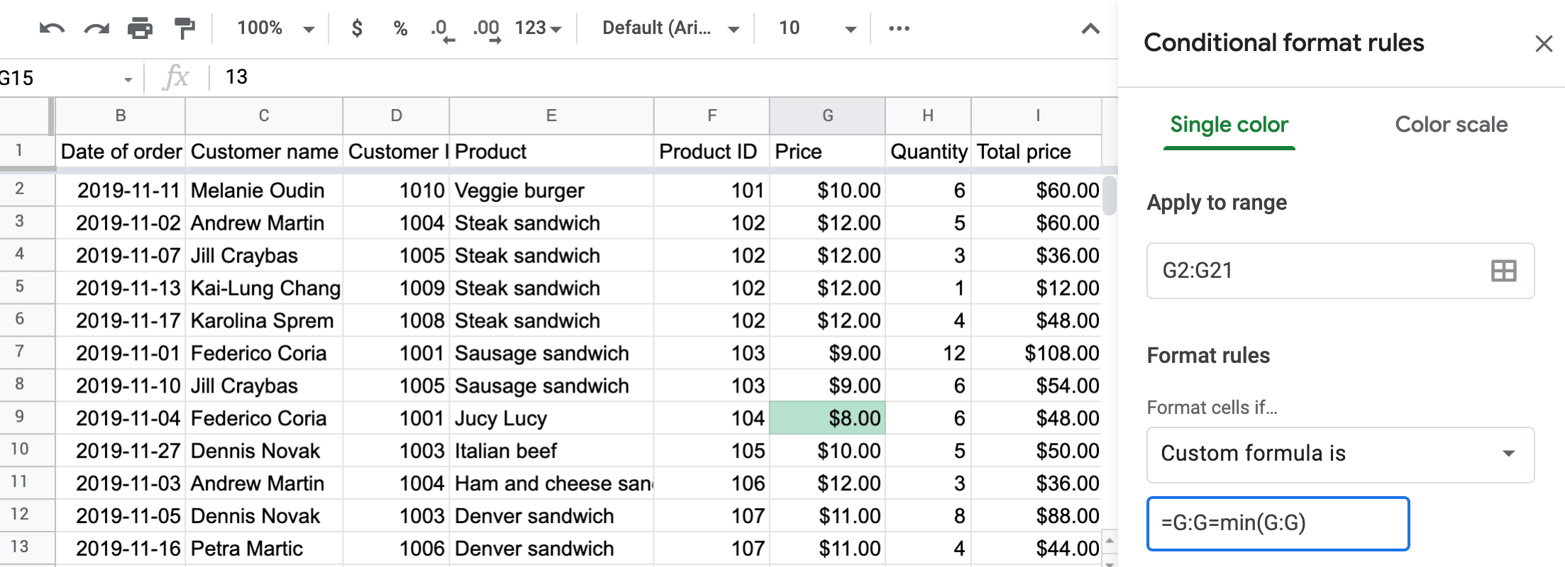
For finding the lowest value, the logic is the same. The formula to type will be

=G:G=min(G:G)

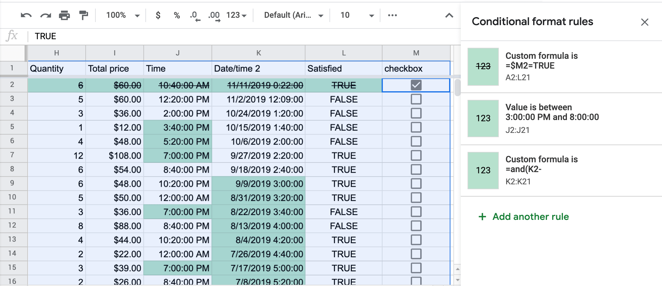
Google Sheets conditional formatting using checkbox

Checkbox and conditional formatting is another cool feature of Google Sheets. If the checkbox is ticked, the entire row changes color or font style. Let's see how to apply it in practice.

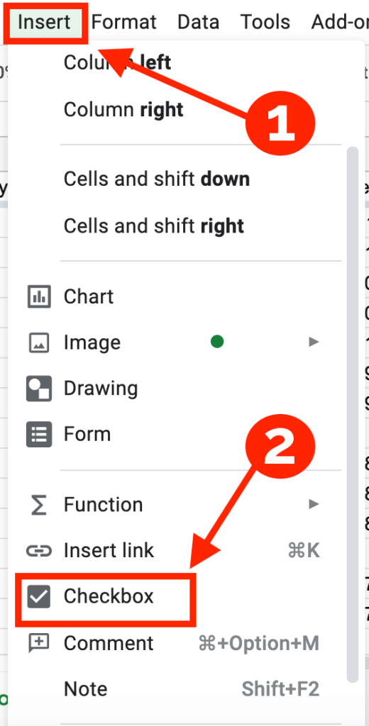
First of all, insert a checkbox from the Insert tab. For that, we created a separate column, H.

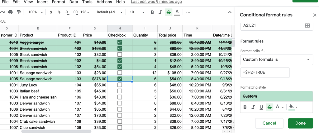
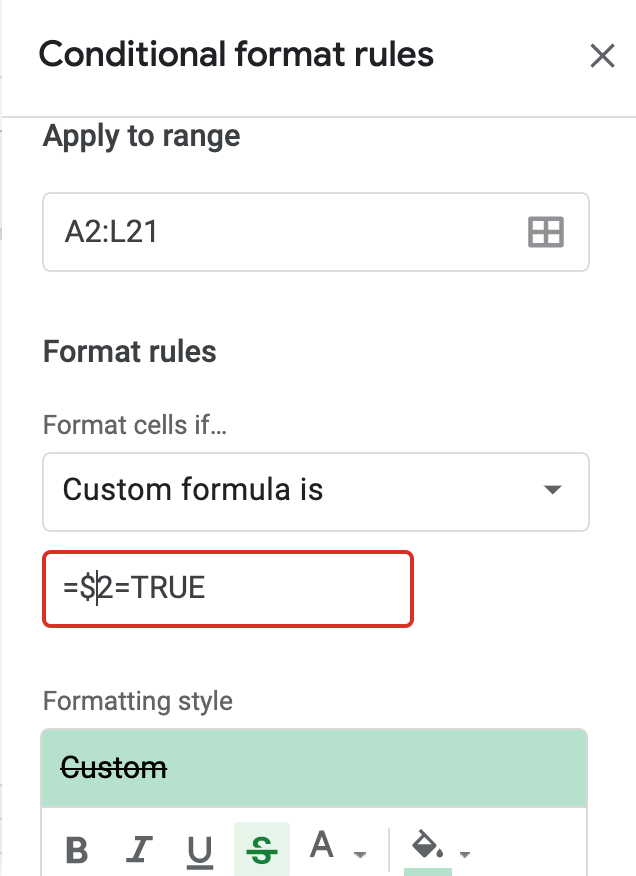
Then, select the range that needs to be conditionally formatted. In our case, it is the whole dataset (A2:L21). And for better visualization, we choose a different color and strikethrough font style when a checkbox is ticked. The last thing to do is select Custom formula is and type

=$H2=TRUE

Now every time you tick your check box, the rule will be applied.

Google Sheets conditional formatting across sheets

Well, it would be great if you could have applied conditional formatting across different sheet tabs. For example, if you highlight the product in one sheet tab, it automatically applies across all sheet tabs without the need for manual editing.

But, unfortunately, conditional format rules only apply to the tab they are entered in. And it is impossible to import them for multiple tabs, let alone different spreadsheets.

Google Sheets conditional formatting not working

If you are also a fan of conditional formatting like we are, and apply it often, or taking your first steps into getting to know this useful tool, you may sometimes face situations when the conditional formatting rule doesn't work. We singled out the four main reasons why this may happen for you:

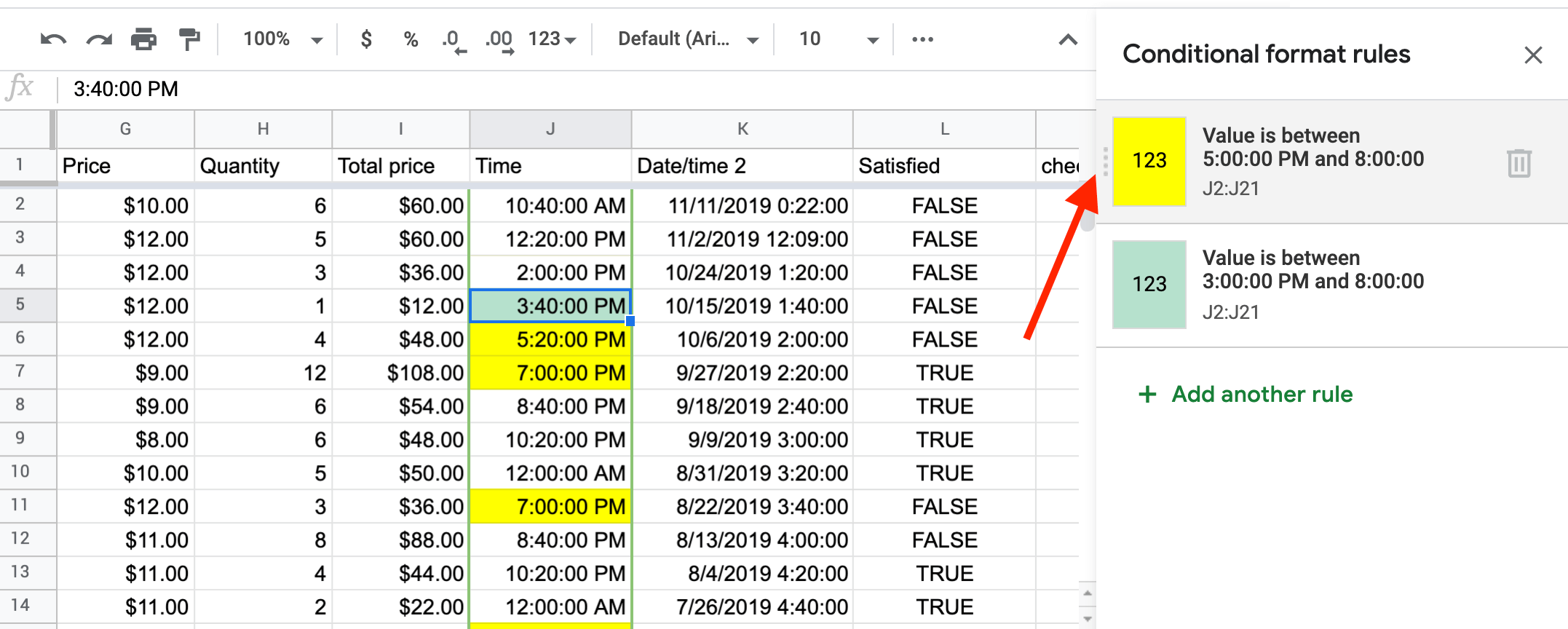
1. The order of your conditional formatting is important. Conditional formatting only applies the first rule (top to bottom) that returns TRUE.

Any other TRUE results won't be calculated. You can change the order by switching the rules around. For that, you need to drag the box using the three dots that appear at the left side.

2. Conditional formatting behaves slightly differently than other Google Sheets formulas. For example, if in the custom formula you enter: =G2<10 and apply it to the range G2:I21, in G2 cell, it will evaluate it exactly as written, G2<10. But in the next cells it will evaluate it as =G3<10, =G4<10 and so on, meaning the conditional formatting will adjust the formula for you.

If you don't want any adjustments you need to use the $ sign. If you use $G$2, it will keep both the row and the column constant across the range. G$2 will only keep the row constant and $G2 will only keep the column constant. To highlight a row based on a single column, you need to use the $G2 option.

3. Unlike in Google Sheets standard formulas, closing parenthesis will not automatically be inserted for you in conditional formatting. You have to be careful with this and manually insert them yourself. In complex formulas, it is often helpful to test the formula in a blank cell to make sure your syntax is correct.

4. Conditional formatting, as we mentioned before, cannot be applied to other tabs in your sheet directly. You have to use the INDIRECT function to reference a different tab within your sheet.

Google Sheets conditional formatting custom formula is invalid

When you use Customer formula is… as part of conditional formatting, you also have to be careful when inputting your formula. Of course, it will not work. Moreover, it will highlight the formula in red, as shown below.

How to remove conditional formatting in Google Sheets

In some cases, you may want to clear the conditional formatting in Google Sheets altogether. This could possibly be the case when you get the data from someone else or you want to start working with your spreadsheet afresh.

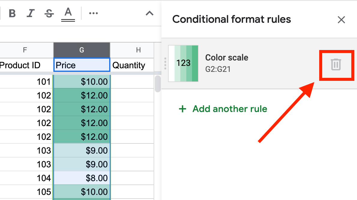
To remove conditional formatting, first, select the range of cells with conditional formatting, then go to Format => Conditional formatting and you will see all the rules that you created in the sidebar. Click the trash bin icon of the rule you want to clear. Conditional formatting will be deleted.

Recap & keep learning the advanced conditional formatting in Google Sheets

No matter what type of project you're working on or what data you're working with, a spreadsheet can be the perfect tool to play with your data and derive meaning from it. With conditional formatting in Google Sheets, you can make your data look visually compelling and add sense to make reports intuitive and reader-friendly. So, keep on learning and applying this great function, and you'll probably find dozens of use cases for conditional formatting.

Back to Blog

Focus on your business

goals while we take care of your data!

Try Coupler.io

inouecrocke.blogspot.com

Source: https://blog.coupler.io/conditional-formatting-google-sheets/

Share this post